Chapter ‍10 Implemented physics

• 10.1 The hard interaction models
• 10.2 The SUSY Les Houches Accord (SLHA) interface
• 10.3 Lepton Collider Beam Spectra
• 10.4 Transverse momentum for ISR photons
• 10.5 Transverse momentum for the EPA approximation
• 10.6 Resonances and continuum
• 10.7 Parton showers and Hadronization

10.1 The hard interaction models

In this section, we give a brief overview over the different incarnations of models for the description of the realm of subatomic particles and their interactions inside WHIZARD. In Sec. ‍10.1.1, the Standard Model (SM) itself and straightforward extensions and modifications thereof in the gauge, fermionic and Higgs sector are described. Then, Sec. ‍10.1.2 gives a list and short description of all genuine beyond the SM models (BSM) that are currently implemented in WHIZARD and its matrix element generator O’Mega. Additional models beyond that can be integrated and handled via the interfaces to external tools like SARAH and FeynRules, or the universal model format UFO, cf. Chap. ‍17.

10.1.1 The Standard Model and friends

10.1.2 Beyond the Standard Model

---

MODEL TYPE	with CKM matrix	trivial CKM
Yukawa test model	---	Test
QED with e,µ,τ,γ	---	QED
QCD with d,u,s,c,b,t,g	---	QCD
Standard Model	SM_CKM	SM
SM with anomalous gauge couplings	SM_ac_CKM	SM_ac
SM with Hgg, Hγγ, Hµµ, He+e−	SM_Higgs_CKM	SM_Higgs
SM with bosonic dim-6 operators	---	SM_dim6
SM with charge 4/3 top	---	SM_top
SM with anomalous top couplings	---	SM_top_anom
SM with anomalous Higgs couplings	---	SM_rx/NoH_rx/SM_ul
SM extensions for VV scattering	---	SSC/AltH/SSC_2/SSC_AltT
SM with Z′	---	Zprime
Two-Higgs Doublet Model	THDM_CKM	THDM
MSSM	MSSM_CKM	MSSM
MSSM with gravitinos	---	MSSM_Grav
NMSSM	NMSSM_CKM	NMSSM
extended SUSY models	---	PSSSM
Littlest Higgs	---	Littlest
Littlest Higgs with ungauged U(1)	---	Littlest_Eta
Littlest Higgs with T parity	---	Littlest_Tpar
Simplest Little Higgs (anomaly-free)	---	Simplest
Simplest Little Higgs (universal)	---	Simplest_univ
SM with graviton	---	Xdim
UED	---	UED
“SQED” with gravitino	---	GravTest
Augmentable SM template	---	Template

Table 10.1: List of models available in WHIZARD. There are pure test models or models implemented for theoretical investigations, a long list of SM variants as well as a large number of BSM models.

---

Strongly Interacting Models and Composite Models

Higgsless models have been studied extensively before the Higgs boson discovery at the LHC Run I in 2012 in order to detect possible loopholes in the electroweak Higgs sector discovery potential of this collider. The Threesite Higgsless Model is one of the simplest incarnations of these models, and was one of the first BSM models beyond SUSY and Little Higgs models that have been implemented in WHIZARD ‍[39]. It is also called the Minimal Higgsless Model (MHM) ‍[40] is a minimal deconstructed Higgsless model which contains only the first resonance in the tower of Kaluza-Klein modes of a Higgsless extra-dimensional model. It is a non-renormalizable, effective theory whose gauge group is an extension of the SM with an extra SU(2) gauge group. The breaking of the extended electroweak gauge symmetry is accomplished by a set of nonlinear sigma fields which represent the effects of physics at a higher scale and make the theory nonrenormalizable. The physical vector boson spectrum contains the usual photon, W^± and Z bosons as well as a W′^± and Z′ boson. Additionally, a new set of heavy fermions are introduced to accompany the new gauge group “site” which mix to form the physical eigenstates. This mixing is controlled by the small mixing parameter є_L which is adjusted to satisfy constraints from precision observables, such as the S parameter ‍[41]. Here, additional weak gauge boson production at the LHC was one of the focus of the studies with WHIZARD ‍[42].

Supersymmetric Models

WHIZARD/O’Mega was the first multi-leg matrix-element/event generator to include the full Minimal Supersymmetric Standard Model (MSSM), and also the NMSSM. The SUSY implementations in WHIZARD have been extensively tested ‍[43, 44], and have been used for many theoretical and experimental studies (some prime examples being ‍[45, 46, 56].

Little Higgs Models

Inofficial models

There have been several models that have been included within the WHIZARD/O’Mega framework but never found their way into the official release series. One famous example is the non-commutative extension of the SM, the NCSM. There have been several studies, e.g. simulations on the s-channel production of a Z boson at the photon collider option of the ILC ‍[49]. Also, the production of electroweak gauge bosons at the LHC in the framework of the NCSM have been studied ‍[50].

10.2 The SUSY Les Houches Accord (SLHA) interface

To be filled in ... ‍[52, 53, 54].

The neutralino sector deserves special attention. After diagonalization of the mass matrix expresssed in terms of the gaugino and higgsino eigenstates, the resulting mass eigenvalues may be either negative or positive. In this case, two procedures can be followed. Either the masses are rendered positive and the associated mixing matrix gets purely imaginary entries or the masses are kept signed, the mixing matrix in this case being real. According to the SLHA agreement, the second option is adopted. For a specific eigenvalue, the phase is absorbed into the definition of the relevant eigenvector, rendering the mass negative. However, WHIZARD has not yet officially tested for negative masses. For external SUSY models (cf. ‍Chap. ‍17) this means, that one must be careful using a SLHA file with explicit factors of the complex unity in the mixing matrix, and on the other hand, real and positive masses for the neutralinos. For the hard-coded SUSY models, this is completely handled internally. Especially Ref. ‍[56] discusses the details of the neutralino (and chargino) mixing matrix.

10.3 Lepton Collider Beam Spectra

For the simulation of lepton collider beam spectra there are two dedicated tools, CIRCE1 and CIRCE2 that have been written as in principle independent tools. Both attempt to describe the details of electron (and positron) beams in a realistic lepton collider environment. Due to the quest for achieving high peak luminosities at e⁺e⁻ machines, the goal is to make the spatial extension of the beam as small as possible but keeping the area of the beam roughly constant. This is achieved by forcing the beams in the final focus into the shape of a quasi-2D bunch. Due to the high charge density in that bunch, the bunch electron distribution is modified by classical electromagnetic radiation, so called beamstrahlung. The two CIRCE packages are intended to perform a simulation of this beamstrahlung and its consequences on the electron beam spectrum as realistic as possible. More details about the two packages can be found in their stand-alone documentations. We will discuss the basic features of lepton-collider beam simulations in the next two sections, including the technicalities of passing simulations of the machine beam setup to WHIZARD. This will be followed by a section on the simulation of photon collider spectra, included for historical reasons.

10.3.1 CIRCE1

While the bunches in a linear collider cross only once, due to their small size they experience a strong beam-beam effect. There is a code to simulate the impact of this effect on luminosity and background, called GuineaPig++ ‍[10, 11, 12]. This takes into account the details of the accelerator, the final focus etc. on the structure of the beam and the main features of the resulting energy spectrum of the electrons and positrons. It offers the state-of-the-art simulation of lepton-collider beam spectra as close as possible to reality. However, for many high-luminosity simulations, event files produced with GuineaPig++ are usually too small, in the sense that not enough independent events are available for physics simulations. Lepton collider beam spectra do peak at the nominal beam energy (√s/2) of the collider, and feature very steeply falling tails. Such steeply falling distributions are very poorly mapped by histogrammed distributions with fixed bin widths.

The main working assumption to handle such spectra are being followed within CIRCE1:

1. The beam spectra for the two beams P₁ and P₂ factorize (here x₁ and x₂ are the energy fractions of the two beams, respectively):

   DP1P2 (x1, x2) = DP1 (x1) · DP2 (x2)

2. The peak is described with a delta distribution, and the tail with a power law:

   D(x) = d · δ(1−x)   +   c · xα  (1−x)β

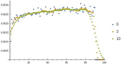
The two powers α and β are the main coefficients that can be tuned in order to describe the spectrum with CIRCE1 as close as possible as the original GuineaPig++ spectrum. More details about how CIRCE1 works and what it does can be found in its own write-up in circe1/share/doc.

10.3.2 CIRCE2

The two conditions listed in 10.3.1 are too restrictive and hence insufficient to describe more complicated lepton-collider beam spectra, as they e.g. occur in the CLIC drive-beam design. Here, the two beams are highly correlated and also a power-law description does not give good enough precision for the tails. To deal with these problems, CIRCE2 starts with a two-dimensional histogram featuring factorized, but variable bin widths in order to simulate the steep parts of the distributions. The limited statistics from too small GuineaPig++ event output files leads to correlated fluctuations that would leave strange artifacts in the distributions. To abandon them, Gaussian filters are applied to smooth out the correlated fluctuations. Here care has to be taken when going from the continuum in x momentum fraction space to the corresponding

---

Figure 10.1: Smoothing the bin at the xe+ = 1 boundary with Gaussian filters of 3 and 10 bins width compared to no smoothing.

---

boundaries: separate smoothing procedures are being applied to the bins in the continuum region and those in the boundary in order to avoid artificial unphysical beam energy spreads. Fig. ‍10.1 shows the smoothing of the distribution for the bin at the x_e⁺ = 1 boundary. The blue dots show the direct GuineaPig++ output comprising the fluctuations due to the low statistics. Gaussian filters with widths of 3 and 10 bins, respectively, have been applied (orange and green dots, resp.). While there is still considerable fluctuation for 3 bin width Gaussian filtering, the distribution is perfectly smooth for 10 bin width. Hence, five bin widths seem a reasonable compromise for histograms with a total of 100 bins. Note that the bins are not equidistant, but shrink with a power law towards the x_e⁻ = 1 boundary on the right hand side of Fig. ‍10.1.

WHIZARD ships (inside its subpackage CIRCE2) with prepared beam spectra ready to be used within CIRCE2 for the ILC beam spectra used in the ILC TDR ‍[13, 14, 15, 16, 17]. These comprise the designed staging energies of 200 GeV, 230 GeV, 250 GeV, 350 GeV, and 500 GeV. Note that all of these spectra up to now do not take polarization of the original beams on the beamstrahlung into account, but are polarization-averaged. For backwards compatibility, also the 500 GeV spectra for the TESLA design ‍[27, 28], here both for polarized and polarization-averaged cases, are included. Correlated spectra for CLIC staging energies like 350 GeV, 1400 GeV and 3000 GeV are not yet (as of version 2.2.4) included in the WHIZARD distribution.

In the following we describe how to obtain such files with the tools included in WHIZARD(resp. CIRCE2). The procedure is equivalent to the so-called lumi-linker construction used by Timothy Barklow (SLAC) together with the legacy version WHIZARD 1.95. The workflow to produce such files is to run GuineaPig++ with the following input parameters:

  do_lumi = 7;
  num_lumi = 100000000;
  num_lumi_eg = 100000000;
  num_lumi_gg = 100000000;

This demands from GuineaPig++ the generation of distributions for the e⁻e⁺, e^∓γ, and γγ components of the beamstrahlung’s spectrum, respectively. These are the files lumi.ee.out, lumi.eg.out, lumi.ge.out, and lumi.gg.out, respectively. These contain pairs (E₁, E₂) of beam energies, not fractions of the original beam energy. Huge event numbers are out in here, as GuineaPig++ will produce only a small fraction due to a very low generation efficiency.

The next step is to transfer these output files from GuineaPig++ into input files used with CIRCE2. This is done by means of the tool circe_tool.opt that is installed together with the WHIZARD main binary and libraries. The user should run this executable with the following input file:

{ file="ilc500/ilc500.circe"                   # to be loaded by WHIZARD
  { design="ILC" roots=500 bins=100 scale=250 # E in [0,1]
    { pid/1=electron pid/2=positron pol=0     # unpolarized e-/e+
      events="ilc500/lumi.ee.out" columns=2   # <= Guinea-Pig
      lumi = 1564.763360                      # <= Guinea-Pig
      iterations = 10                         # adapting bins
      smooth = 5 [0,1) [0,1)                  # Gaussian filter 5 bins
      smooth = 5 [1] [0,1) smooth = 5 [0,1) [1] } } }

The first line defines the output file, that later can be read in into the beamstrahlung’s description of WHIZARD (cf. below). Then, in the second line the design of the collider (here: ILC for 500 GeV center-of-mass energy, with the number of bins) is specified. The next line tells the tool to take the unpolarized case, then the GuineaPig++ parameters (event file and luminosity) are set. In the last three lines, details concerning the adaptation of the simulation as well as the smoothing procedure are being specified: the number of iterations in the adaptation procedure, and for the smoothing with the Gaussian filter first in the continuum and then at the two edges of the spectrum. For more details confer the documentation in the CIRCE2 subpackage.

This produces the corresponding input files that can be used within WHIZARD to describe beamstrahlung for lepton colliders, using a SINDARIN input file like:

        beams = e1, E1 => circe2
        $circe2_file = "ilc500.circe"
        $circe2_design = "ILC"
        ?circe2_polarized = false

10.3.3 Photon Collider Spectra

For details confer the complete write-up of the CIRCE2 subpackage.

10.4 Transverse momentum for ISR photons

The structure functions that describe the splitting of a beam particle into a particle pair, of which one enters the hard interaction and the other one is radiated, are defined and evaluated in the strict collinear approximation. In particular, this holds for the ISR structure function which describes the radiation of photons off a charged particle in the initial state.

The ISR structure function that is used by WHIZARD is understood to be inclusive, i.e., it implicitly contains an integration over transverse momentum. This approach is to be used for computing a total cross section via integrate. In WHIZARD, it is possible to unfold this integration, as a transformation that is applied by simulate step, event by event. The resulting modified events will show a proper logarithmic momentum-transfer (Q²) distribution for the radiated photons. The recoil is applied to the hard-interaction system, such that four-momentum and √ŝ are conserved. The distribution is cut off by Q_max² (cf. isr_q_max) for large momentum transfer, and smoothly by the parton mass (cf. isr_mass) for small momentum transfer.

To activate this modification, set

  ?isr_handler = true
  $isr_handler_mode = "recoil"

before, or as an option to, the simulate command.

Limitations: the current implementation of the p_T modification works only for the symmetric double-ISR case, i.e., both beams have to be charged particles with identical mass (e.g., e⁺e⁻). The mode recoil generates exactly one photon per beam, i.e., it modifies the momentum of the single collinear photon that the ISR structure function implementation produces, for each beam. (It is foreseen that further modes or options will allow to generate multiple photons. Alternatively, the PYTHIA shower can be used to simulate multiple photons radiated from the initial state.)

10.5 Transverse momentum for the EPA approximation

For the equivalent-photon approximation (EPA), which is also defined in the collinear limit, recoil momentum can be inserted into generated events in an entirely analogous way. The appropriate settings are

  ?epa_handler = true
  $epa_handler_mode = "recoil"

Limitations: as for ISR, the current implementation of the p_T modification works only for the symmetric double-EPA case. Both incoming particles of the hard process must be photons, while both beams must be charged particles with identical mass (e.g., e⁺e⁻). Furthermore, the current implementation does not respect the kinematical limit parameter epa_q_min, it has to be set to zero. In effect, the lower Q² cutoff is determined by the beam-particle mass epa_mass, and the upper cutoff is either given by Q_max (the parameter epa_q_max), or by the limit √s if this is not set.

It is possible to combine the ISR and EPA handlers, for processes where ISR is active for one of the beams, EPA for the other beam. For this scenario to work, both handler switches must be on, and both mode strings must coincide. The parameters are set separately for ISR and EPA, as described above.

10.6 Resonances and continuum

10.6.1 Complete matrix elements

Many elementary physical processes are composed of contributions that can be qualified as (multiply) resonant or continuum. For instance, the amplitude for the process e⁺e⁻→ qq qq, evaluated at tree level in perturbation theory, contains Feynman diagrams with zero, one, or two W and Z bosons as virtual lines. If the kinematical constraints allow this, two vector bosons can become simultaneously on-shell in part of phase space. To a first approximation, this situation is understood as W⁺W⁻ or ZZ production with subsequent decay. The kinematical distributions show distinct resonances in the quark-pair spectra. Other graphs contain only one s-channel W/Z boson, or none at all, such as graphs with qq production and subsequent gluon radiation, splitting into another qq pair.

A WHIZARD declaration of the form

        process q4 = e1, E1 => u, U, d, D

produces the full set of graphs for the selected final state, which after squaring and integrating yields the exact tree-level result for the process. The result contains all doubly and singly resonant parts, with correct resonance shapes, as well as the continuum contribution and all interference. This is, to given order in perturbation theory, the best possible approximation to the true result.

10.6.2 Processes restricted to resonances

For an intuitive separation of a two-boson “signal” contribution, it is possible to restrict the set of graphs to a certain intermediate state. For instance, the declaration

  process q4_zz = e1, E1 => u, U, d, D { $restrictions = "3+4~Z && 5+6~Z" }

generates an amplitude that contains only those Feynman graphs where the specified quarks are connected to a Z virtual line. The result may be understood as ZZ production with subsequent decay, where the Z resonances exhibit a Breit-Wigner shape. Combining this with the analogous W⁺W⁻ restricted process, the user can generate “signal” processes.

Adding both “signal” cross sections WW and ZZ will result in a reasonable approximation to the exact tree-level cross section. The amplitude misses the single-resonant and continuum contributions, and the squared amplitude misses the interference terms, however. More importantly, the restricted processes as such are not gauge-invariant (with respect to the electroweak gauge group), and they are no longer dominant away from resonant kinematics. We therefore strongly recommend that such restricted processes are always accompanied by a cut setup that restricts the kinematics to an approximately on-shell pattern for both resonances. For instance:

  cuts = all 85 GeV < M < 95 GeV [u:U]
     and all 85 GeV < M < 95 GeV [d:D]

In this region, the gauge-dependent and continuum contributions are strictly subdominant. Away from the resonance(s), the results for a restricted process are meaningless, and the full process has to be computed instead.

10.6.3 Factorized processes

Another method for obtaining the signal contribution is a proper factorization into resonance production and decay. We would have to generate a production process and two decay processes:

        process z_uu = Z => u, U
        process z_dd = Z => d, D
        process zz = e1, E1 => Z, Z

All three processes must be integrated. The integration results are partial decay widths and the ZZ production cross section, respectively. (Note that cut expressions in SINDARIN apply to all integrations, so make sure that no production-process cuts are active when integrating the decay processes.)

During a later event-generation step, the Z decays can then be activated by declaring the Z as unstable,

        unstable Z (z_uu, z_dd)

and then simulating the production process

        simulate (zz)

The generated events will consist of four-fermion final states, including all combinations of both decay modes. It is important to note that in this setup, the invariant uū and dd masses will be always exactly equal to the Z mass. There is no Breit-Wigner shape involved. However, in this approximation the results are gauge-invariant, as there is no off-shell contribution involved.

For further details on factorized processes and spin correlations, cf. Sec. ‍5.8.2.

10.6.4 Resonance insertion in the event record

From the above discussion, we may conclude that it is always preferable to compute the complete process for a given final state, as long as this is computationally feasible. However, in the simulation step this approach also has a drawback. Namely, if a parton-shower module (see below) is switched on, the parton-shower algorithm relies on event details in order to determine the radiation pattern of gluons and further splitting. In the generated event records, the full-process events carry the signature of non-resonant continuum production with no intermediate resonances. The parton shower will thus start the evolution at the process energy scale, the total available energy. By contrast, for an electroweak production and decay process, the evolution should start only at the vector boson mass, m_Z. In effect, even though the resonant contribution of WW and ZZ constitutes the bulk of the cross section, the radiation pattern follows the dynamics of four-quark continuum production. In general, the number of radiated hadrons will be too high.

---

Figure 10.2: The process e+e− → jjjj at 250 GeV center-of-mass energy is compared transferring the partonic events naively to the parton shower, i.e. without respecting any intermediate resonances (red lines). The blue lines show the process factorized into WW production and decay, where the shower knows the origin of the two jet pairs. The orange and dark green lines show the resonance treatment as mentioned in the text, with resonance_on_shell_limit = 1 and = 4, respectively. PYTHIA6 parton shower and hadronization with the OPAL tune have been used. The observables are: photon energy distribution and number of charged tracks (upper line left/right, number of hadrons and total number of particles (middle left/right), and number of photons and neutral particles (lower line left/right).

---

To overcome this problem, there is a refinement of the process description available in WHIZARD. By modifying the process declaration to

  ?resonance_history = true
  resonance_on_shell_limit = 4
  process q4 = e1, E1 => u, U, d, D

we advise the program to produce not just the complete matrix element, but also all possible restricted matrix elements containing resonant intermediate states. This has no effect at all on the integration step, and thus on the total cross section.

However, when subsequently events are generated with this setting, the program checks, for each event, the kinematics and determines the set of potentially resonant contributions. The criterion is whether the off-shellness of a particular would-be resonance is less than the resonance width multiplied by the value of resonance_on_shell_limit (default value =4). For the set of resonance histories which pass this criterion (which can be empty), their respective squared matrix element is related to the full-process matrix element. The ratio is interpreted as a probability. The random-number generator then selects one or none of the resonance histories, and modifies the event record accordingly. In effect, for an appropriate fraction of the events, depending on the kinematics, the parton-shower module is provided with resonance information, so it can adjust the radiation pattern accordingly.

It has to be mentioned that generating the matrix-element code for all possible resonance histories takes additional computing resources. In the current default setup, this feature is switched off. It has to be explicitly activated via the ?resonance_history flag.

Also, the feature can be activated or deactivated individually for each process, such as in

  ?resonance_history = true
  process q4_with_res = e1, E1 => u, U, d, D  { ?resonance_history = true }
  process q4_wo_res   = e1, E1 => u, U, d, D  { ?resonance_history = false }

If the flag is false for a process, no resonance code will be generated. Similarly, the flag has to be globally or locally active when simulate is called, such that the feature takes effect for event generation.

There are two additional parameters that can fine-tune the conditions for resonance insertion in the event record. Firstly, the parameter resonance_on_shell_turnoff, if nonzero, enables a Gaussian suppression of the probability for resonance insertion. For instance, setting

  ?resonance_history = true
  resonance_on_shell_turnoff = 4
  resonance_on_shell_limit = 8

will reduce the probability for the event to be qualified as resonant by e⁻¹= 37 % if the kinematics is off-shell by four units of the width, and by e⁻⁴=2 % at eight units of the width. Beyond this point, the setting of the resonance_on_shell_limit parameter eliminates resonance insertion altogether. In effect, the resonance-background transition is realized in a smooth way. Secondly, within the resonant-kinematics range the probability for qualifying the event as background can be reduced by the parameter resonance_background_factor (default value =1) to a number between zero and one. Setting this to zero means that the event will be necessarily qualified as resonant, if it falls within the resonant-kinematics range.

Note that if an event, by the above mechanism, is identified as following a certain resonance history, the assigned color flow will be chosen to match the resonance history, not the complete matrix element. This may result in a reassignment of color flow with respect to the original partonic event.

Finally, we mention the order of execution: any additional matrix element code is compiled and linked when compile is executed for the processes in question. If this command is omitted, the simulate command will trigger compilation.

10.7 Parton showers and Hadronization

In order to produce sensible events, final state QCD (and also QED) radiation has to be considered as well as the binding of strongly interacting partons into mesons and baryons. Furthermore, final state hadronic resonances undergo subsequent decays into those particles showing up in (or traversing) the detector. The latter are mostly pions, kaons, photons, electrons and muons.

The physics associated with these topics can be divided into the perturbative part which is the regime of the parton shower, and the non-perturbative part which is the regime for the hadronization. WHIZARD comes with its own two different parton shower implementations, an analytic and a so-called k_T-ordered parton shower that will be detailed in the next section.

Note that in general it is not advisable to use different shower and hadronization methods, or in other words, when using shower and hadronization methods from different programs these would have to be tuned together again with the corresponding data.

Parton showers are approximations to full matrix elements taking only the leading color flow into account, and neglecting all interferences between different amplitudes leading to the same exclusive final state. They rely on the QCD (and QED) splitting functions to describe the emissions of partons off other partons. This is encoded in the so-called Sudakov form factor ‍[29]:

This gives the probability for a parton to evolve from scale t₂ to t₁ without any further emissions of partons. t is the evolution parameter of the shower, which can be a parton energy, an emission angle, a virtuality, a transverse momentum etc. The variable z relates the two partons after the branching, with the most common choice being the ratio of energies of the parton after and before the branching. For final-state radiation brachings occur after the hard interaction, the evolution of the shower starts at the scale of the hard interaction, t ∼ ŝ, down to a cut-off scale t = t_cut that marks the transition to the non-perturbative regime of hadronization. In the space-like evolution for the initial-state shower, the evolution is from a cut-off representing the factorization scale for the parton distribution functions (PDFs) to the inverse of the hard process scale, −ŝ. Technically, this evolution is then backwards in (shower) time ‍[30], leading to the necessity to include the PDFs in the Sudakov factors.

The main switches for the shower and hadronization which are realized as transformations on the partonic events within WHIZARD are ?allow_shower and ?allow_hadronization, which are true by default and only there for technical reasons. Next, different shower and hadronization methods can be chosen within WHIZARD:

  $shower_method = "WHIZARD"
  $hadronization_method = "PYTHIA6"

The snippet above shows the default choices in WHIZARD  namely WHIZARD’s intrinsic parton shower, but PYTHIA6 as hadronization tool. (Note that WHIZARD does not have its own hadronization module yet.) The usage of PYTHIA6 for showering and hadronization will be explained in Sec. ‍10.7.3, while the two different implementations of the WHIZARD homebrew parton showers are discussed in Sec. ‍10.7.1 and ‍10.7.2, respectively.

10.7.1 The k_T-ordered parton shower

10.7.2 The analytic parton shower

10.7.3 Parton shower and hadronization from PYTHIA6

Development of the PYTHIA6 generator for parton shower and hadronization (the Fortran version) has been discontinued by the authors several years ago. Hence, the final release of that program is frozen. This allowed to ship this final version, v6.427, with the WHIZARD distribution without the need of updating it all the time. One of the main reasons for that inclusion – besides having the standard tool for showering and hadronization for decays at hand – is to allow for backwards validation within WHIZARD particularly for the event samples generated for the development of linear collider physics: first for TESLA, JLC and NLC, and later on for the Conceptual and Technical Design Report for ILC, for the Conceptual Design Report for CLIC as well as for the Letters of Intent for the LC detectors, ILD and SiD.

Usually, an external parton shower and hadronization program (PS) is steered via the transfer of event files that are given to the PS via LHE events, while the PS program then produces hadron level events, usually in HepMC format. These can then be directed towards a full or fast detector simulation program. As PYTHIA6 has been completely integrated inside the WHIZARD framework, the showered or more general hadron level events can be returned to and kept inside WHIZARD’s internal event record, and hence be used in WHIZARD’s internal event analysis. In that way, the events can be also written out in event formats that are not supported by PYTHIA6, e.g. LCIO via the output capabilities of WHIZARD.

There are several switches to directly steer PYTHIA6 (the values in brackets correspond to the PYTHIA6 variables):

  ps_mass_cutoff = 1 GeV                  [PARJ(82)]
  ps_fsr_lambda = 0.29 GeV                [PARP(72)]
  ps_isr_lambda = 0.29 GeV                [PARP(61)]
  ps_max_n_flavors = 5                    [MSTJ(45)]
  ?ps_isr_alphas_running = true           [MSTP(64)]
  ?ps_fsr_alphas_running = true           [MSTJ(44)]
  ps_fixed_alphas = 0.2                   [PARU(111)]
  ?ps_isr_angular_ordered = true          [MSTP(62)]
  ps_isr_primordial_kt_width = 1.5 GeV    [PARP(91)]
  ps_isr_primordial_kt_cutoff = 5.0 GeV   [PARP(93)]
  ps_isr_z_cutoff = 0.999                 [1-PARP(66)]
  ps_isr_minenergy = 2 GeV                [PARP(65)]
  ?ps_isr_only_onshell_emitted_partons =
        true                              [MSTP(63)]

The values given above are the default values. The first value corresponds to the PYTHIA6 parameter PARJ(82), its squared being the minimal virtuality that is allowed for the parton shower, i.e. the cross-over to the hadronization. The same parameter is used also for the WHIZARD showers. ps_fsr_lambda is the equivalent of PARP(72) and is the Λ_QCD for the final state shower. The corresponding variable for the initial state shower is called PARP(61) in PYTHIA6. By the next variable (MSTJ(45)), the maximal number of flavors produced in splittings in the shower is given, together with the number of active flavors in the running of α_s. ?ps_isr_alphas_running which corresponds to MSTP(64) in PYTHIA6 determines whether or net a running α_s is taken in the space-like initial state showers. The same variable for the final state shower is MSTJ(44). For fixed α_s, the default value is given by ps_fixed_alpha, corresponding to PARU(111). MSTP(62) determines whether the ISR shower is angular order, i.e. whether angles are increasing towards the hard interaction. This is per default true, and set in the variable ?ps_isr_angular_ordered. The width of the distribution for the primordial (intrinsic) k_T distribution (which is a non-perturbative quantity) is the PYTHIA6 variable PARP(91), while in WHIZARD it is given by pythia_isr_primordial_kt_width. The next variable (PARP(93) gives the upper cutoff for that distribution, which is 5 GeV per default. For splitting in space-like showers, there is a cutoff on the z variable named ps_isr_z_cutoff in WHIZARD. This corresponds to one minus the value of the PYTHIA6 parameter PARP(66). PARP(65), on the other hand, gives the minimal (effective) energy for a time-like or on-shell emitted parton on a space-like QCD shower, given by the SINDARIN parameter ps_isr_minenergy. Whether or not partons emitted from space-like showers are allowed to be only on-shell is given by ?ps_isr_only_onshell_emitted_partons, MSTP(63) in PYTHIA6 language. For more details confer the PYTHIA6 manual ‍[31].

Any other non-standard PYTHIA6 parameter can be fed into the parton shower via the string variable

  $ps_PYTHIA_PYGIVE = "...."

Variables set here get preference over the ones set explicitly by dedicated SINDARIN commands. For example, the OPAL tune for hadronic final states can be set via:

  $ps_PYTHIA_PYGIVE = "MSTJ(28)=0; PMAS(25,1)=120.; PMAS(25,2)=0.3605E-02; MSTJ(41)=2;
   MSTU(22)=2000; PARJ(21)=0.40000; PARJ(41)=0.11000; PARJ(42)=0.52000; PARJ(81)=0.25000;
   PARJ(82)=1.90000; MSTJ(11)=3; PARJ(54)=-0.03100; PARJ(55)=-0.00200; PARJ(1)=0.08500;
   PARJ(3)=0.45000; PARJ(4)=0.02500; PARJ(2)=0.31000; PARJ(11)=0.60000; PARJ(12)=0.40000;
   PARJ(13)=0.72000; PARJ(14)=0.43000; PARJ(15)=0.08000; PARJ(16)=0.08000;
   PARJ(17)=0.17000; MSTP(3)=1;MSTP(71)=1"

A very common error that appears quite often when using PYTHIA6 for SUSY or any other model having a stable particle that serves as a possible Dark Matter candidate, is the following warning/error message:

     Advisory warning type 3 given after        0 PYEXEC calls:
     (PYRESD:) Failed to decay particle  1000022 with mass   15.000
******************************************************************************
******************************************************************************
*** FATAL ERROR: Simulation: failed to generate valid event after 10000 tries
******************************************************************************
******************************************************************************

In that case, PYTHIA6 gets a stable particle (here the lightest neutralino with the PDG code 1000022) handed over and does not know what to do with it. Particularly, it wants to treat it as a heavy resonance which should be decayed, but does not know how do that. After a certain number of tries (in the example abobe 10k), WHIZARD ends with a fatal error telling the user that the event transformation for the parton shower in the simulation has failed without producing a valid event. The solution to work around that problem is to let PYTHIA6 know that the neutralino (or any other DM candidate) is stable by means of

  $ps_PYTHIA_PYGIVE = "MDCY(C1000022,1)=0"

Here, 1000022 has to be replaced by the stable dark matter candidate or long-lived particle in the user’s favorite model. Also note that with other options being passed to PYTHIA6  the MDCY option above has to be added to an existing $ps_PYTHIA_PYGIVE command separated by a semicolon.

10.7.4 Parton shower and hadronization from PYTHIA8

10.7.5 Other tools for parton shower and hadronization

10.7.6 Loop-induced processes

In order to steer loop-induced processes the usage of the OLP OpenLoopsis required. Information on the interface and setting up this program can be found in Sec. ‍9.5 and Sec. ‍5.11.1. Furthermore the following settings should be observed

• Choose the model SM_Higgs to allow vertices such as gg → H.
• Use $method="openloops" for the loop-squared amplitudes.
• Set the coupling powers alpha_power and alphas_power corresponding to those of loop-squared amplitudes of the process.